If quantum particles sometimes behave as waves (see the double slit experiment for more details) it’s fair to expect wave-like phenomena play a role in quantum physics and, hence, in quantum computing.
(Quantum) Interference is such a phenomenon. It builds on our notion of Superposition and helps us understand why many quantum algorithms work the way they do.
What is Interference?
In (non-quantum) physics, whenever two waves overlap we encounter Interference.
Let’s imagine a perfectly calm pond as an example. Every point on the surface of this pond has the same height (f.e. as measured by its distance to sea level).
If we drop a rock into our pond, the water starts to wave. Different points on the surface of our pond begin to have different heights. Some are lower than before, while others exceed their previous state.
If we drop a second rock into our pond, the waves generated by each rock begin to overlap. For all spots where both waves have either a peak or a valley, they amplify each other. Peaks become higher and valleys become lower. This phenomenon is referred to as constructive Interference.
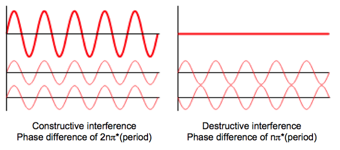
Whenever a peak in one wave overlaps with a valley in another, they cancel each other out. The resulting height is closer to the reference point than either the peak or the valley. The absolute deviation from the baseline is lower. The resulting spot has become less wave-y.
Since we are used to smooth sinus-shaped waves whenever we talk about water, it is worth pointing out that waves don’t have to be sinusoidal.
In audio processing, for example, waves can be shaped like squares, triangles, sawteeth, or pretty much whatever you can think of. (Check out this Wikipedia page for some audio samples of different waveforms)
In general, a wave is a disturbance from a point of equilibrium.
In our example, the equilibrium was the height of any surface point of the pond when it was calm. The disturbance is the deviation in height from this reference point as we throw in the rocks.
In sound, the disturbance is a vibration traveling through a medium such as air. In radio waves, it’s the force of an electromagnetic field. In quantum mechanics, as weird as it may sound, it’s probability…
What’s waving in quantum computing?
The double slit experiment showed us that under certain conditions quantum objects such as electrons behave like waves.
While the Schrödinger equation, derived by Erwin Schrödinger in 1925/26, explains how these waves behave, even Schrödinger himself wasn’t sure what they were made of.
In 1926, Max Born resolved this question by postulating the Born rule. According to Born, if we square the absolute value of the wave, we get the probability of measuring the quantum property in a certain state.
If the wave function refers to the position of a particle in a box, then the squared wave function indicates the probability of finding the particle at each point in space.
In contrast to the probabilities we obtain by squaring the wave function, the wave function itself is described in terms of probability amplitudes.
Mathematically speaking, the probability amplitude of the property of a quantum particle in a specific state is a complex number \alpha so that \alpha \element \C and 0 ≤ | \alpha | ≤ 1.
Let’s look at an example.
Quantum Interference in action
In What is Entanglement we introduced the example of a kindergarten to illustrate how entanglement relates to probability. Let’s revisit that example and focus on a single child.
At any point, the child can be in a good mood 😇 or in a bad mood 😈.
If we assume this kid behaves like a quantum particle, we can describe its state as \( |mood> = \alpha |good> + \beta |bad> \) where \( \alpha, \beta \epsilon \mathbb{C} \) and \(|\alpha|^2 + |\beta|^2 = 1\).
\(\alpha\) and \(\beta\) are the probability amplitudes of each possible state the child can be in if we do not observe it. Once we enter the room, we see a happy child in \(|\alpha|^2 \)% of the time, and a bad-mood child in \(|\beta|^2\) % of all cases.
Coming back to Quantum Interference…
Recall, that a wave is a disturbance from a point of equilibrium.
In our pond from earlier, the equilibrium state was the level of the surface as the pond was calm. The disturbance was any point on the surface that was higher or lower than this reference point.
Interference occurs whenever two waves (hence, two disturbances) overlap.
In the case of the property of a quantum particle, the point of equilibrium is a probability amplitude of 0. In other words: our default is non-existence. If the probability amplitude is 0, then so is the corresponding probability.
The wave/disturbance, in this case, is any probability amplitude different from 0.
Since probability amplitudes can be negative or positive (in contrast to “normal” probability), they can interfere similarly with water waves.
Let’s say, that the child arrives at our kindergarten in a Superposition state of \( |mood> = \frac{1}{\sqrt{2}} |good> + \frac{1}{\sqrt{2}} |bad> \). The child has only been coming to our kindergarten for a few days, so it occasionally misses its parents and acts up.
If we were to meet it now, we would find it in a good mood with a probability of \(|\frac{1}{\sqrt{2}}|^2 = 0.5\) and in a bad mood with a probability of \(|\frac{1}{\sqrt{2}}|^2 = 0.5\) respectively.
To make our (and their) lives easier, we placed a chocolate bar 🍫 near the entrance, the child’s favorite snack. Depending on the state the child is in when it finds the snack, this can either make it happy or sad (as it might associate chocolate with home).
Based on the state the child is in when receiving the snack, its new state can be derived according to the following formulas*:
\(chocolate |good> = \frac{1}{\sqrt{2}} |good> + \frac{1}{\sqrt{2}} |bad>\)
\(chocolate |bad> = \frac{1}{\sqrt{2}} |good> – \frac{1}{\sqrt{2}} |bad>\)
Regardless of whether the child was in a good or a bad mood when receiving the chocolate, if we observe it afterward it is equally likely to be either happy or sad, since \(|\frac{1}{\sqrt{2}}|^2 = |-\frac{1}{\sqrt{2}}|^2 = 0.5\).
* Purely by coincidence, this transformation closely resembles one of the most important quantum gates, the Hadamard gate.
Interesting things happen when we apply our transformation (🍫) to a superposition state of the two.
Since all operations in quantum computing are distributive, we can distribute the operation onto each of the component states of the superposition.
\(chocolate (\frac{1}{\sqrt{2}} |good> + \frac{1}{\sqrt{2}} |bad>)\)
\( = \frac{1}{\sqrt{2}} chocolate |good> + \frac{1}{\sqrt{2}} chocolate |bad>\)
\(= \frac{1}{\sqrt{2}} ( \frac{1}{\sqrt{2}} |good> + \frac{1}{\sqrt{2}} |bad>) \times \frac{1}{\sqrt{2}} (\frac{1}{\sqrt{2}} |good> – \frac{1}{\sqrt{2}} |bad>)\)
\(= \frac{1}{2} |good> + \frac{1}{2} |bad> + \frac{1}{2} |good> – \frac{1}{2} |bad>\)
\(= 2 \times \frac{1}{2} |good>\)
\(= |good>\)
Each component state of the superposition has been mapped to a superposition of two states. Based on the signs of the corresponding coefficients, these waves could interfere either destructively or constructively.
Since the coefficients of both |😇> were positive, they interfered constructively, increasing the absolute value of the corresponding probability amplitude. Both |😈> waves, however, had opposing-sign coefficients. They interfered destructively and canceled each other out.
How is Quantum Interference used?
Quantum Interference is at the core of many quantum algorithms such as the Quantum Fourier Transform or Grover’s Algorithm.
In Grover’s Algorithm, a superposition of possible solutions to a problem is modified by an oracle function, which changes the sign of the state that solves the problem (s. this article). Each state in this superposition is then mapped to a superposition of all states.
Based on how the Diffusion operator is defined in the algorithm, constructive Interference increases the probability of the marked state among all possibilities upon measurement. Destructive Interference, in contrast, reduces the probability (amplitudes) of all other states. The previous change in sign causes different Interference patterns for different states.
In the Quantum Fourier Transform, each state of the input sample is mapped to a superposition of states in the frequency domain. These states then interfere, resulting in the summation contained in the (non-quantum) definition of the Discrete Fourier Transform.
In general, Quantum Interference can occur whenever we apply an operation to a superposition state, that maps each of the component states of the superposition to a superposition of its own. That’s what happened in our chocolate-craving kindergartener example.
Summary
In quantum computing, probability amplitudes describe the behavior of quantum particles and their properties. These probability amplitudes are similar to the probabilities we know from everyday life, except they can also assume negative and complex values.
If two probability amplitudes for the same state overlap, they can either amplify or dampen each other. This phenomenon is referred to as (quantum) Interference and lies at the core of quantum algorithms such as the Quantum Fourier Transform or Grover’s Algorithm.