What is the Optimal Number of Iterations in Grover’s Algorithm?
Grover’s algorithm promises a quadratic speedup on the unstructured search problem.
To find a specific value among \( N \) possible values, a classical computer would have to check up to \( N – 1 \) candidates. This results in a time complexity of \( O(N) \) .
Grover’s algorithm, in turn, returns the desired value in \( O(\sqrt{N}) \) steps with a probability of up to 100%.
In a previous post, we explored Grover’s algorithm in detail and described the role that quantum parallelism plays in achieving the speedup.
In this post, we will look at the calculation that was used to derive the exact speed up of \( \sqrt{N} \) .
Enjoy!
A State of States
Grover’s algorithm begins by placing the quantum computer in an equal superposition of all possible states. With \( n \) qubits and \( N=2^n \) base states, the initial superposition state is \( |s> = \frac{1}{\sqrt{N}} \sum_{i=0}^{N-1} |i> \).
Note, that the choice of base state is more or less arbitrary. We generally use \( |0…00>, |0…01>, |0…10>, … \) as the base states to represent our computations, but that need not be the case.
Any set of states can be chosen as base states as long as the states are orthogonal and the set is complete, i.e., every state in the N-dimensional Hilbert space can be expressed as a linear combination of the chosen base states.
In the context of Grover’s algorithm, there are two types of states we care about: The states that form a solution to the search problem and the rest.
With \( M \) solutions to our problem, the state that combines all of these solutions can be expressed as \( |w> = \frac{1}{\sqrt{M}} \sum_{i \epsilon M} |i> \). It is an equal superposition of all \( M \) solutions.
The state that contains all non-solutions, can be expressed as \( |w’> = \frac{1}{\sqrt{N-M}} \sum_{i \epsilon N \setminus M} |i> \). It contains an equal superposition of all \( N-M \) states that do not solve the search problem.
Because \( |w> \) and \( |w’> \) are orthogonal and can be used to describe every state reachable in Grover’s algorithm (more on that in a second), they form a feasible choice for our basis of computation.
The state of the system in Grover’s algorithm can therefore be written as a superposition \(|s> = a |w> + b |w’>\) where \(|a|^2 + |b|^2 = 1\).
A Geometric Interpretation of Superposition
Let’s create a figure with two axes that correspond to \(|w>\) and \(|w’>\).
Because \(|w>\) and \(|w’>\) are orthogonal, the axes meet at a right angle.
The initial superposition state created at the beginning of Grover’s algorithm, can be written as a superposition state of \(|w>\) and \(|w’>\), our alternative basis.
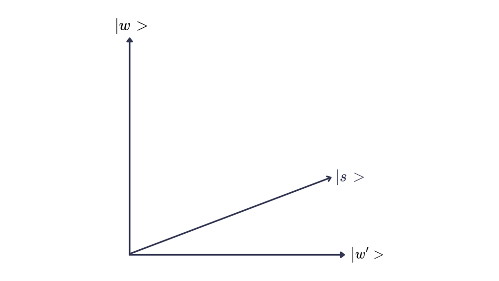
Figure 1 shows the state of the system before the Oracle and Diffusion operators are applied.
The weight that \(|w>\) and \(|w’>\) have in the initial superposition, can be calculated by projecting the state \(|s>\) onto the corresponding axis.
The weight of \(|w>\) in the superposition corresponds to the the height of the vector of \(|s>\) in Figure 1.
Each of the \(M\) correct states has a probability amplitude of \(\frac{1}{\sqrt{N}}\) in \(|s>\) and a corresponding probability amplitude of \(\frac{1}{\sqrt{M}}\) in \(|w>\).
Together, the correct states have a probability amplitude of \(M * \frac{1}{\sqrt{N}} * \frac{1}{\sqrt{M}} = \frac{1}{\sqrt{N}} * \frac{M}{\sqrt{M}} = \frac{\sqrt{M}}{\sqrt{N}}\).
Likewise, the probability amplitude of the incorrect states in the initial superposition becomes \(\frac{\sqrt{N – M}}{\sqrt{N}}\).
The state as a whole can therefore be written as \(|s> = \frac{\sqrt{M}}{\sqrt{N}} |w> + \frac{\sqrt{N – M}}{\sqrt{N}} |w’>\).
From Weights to Angles
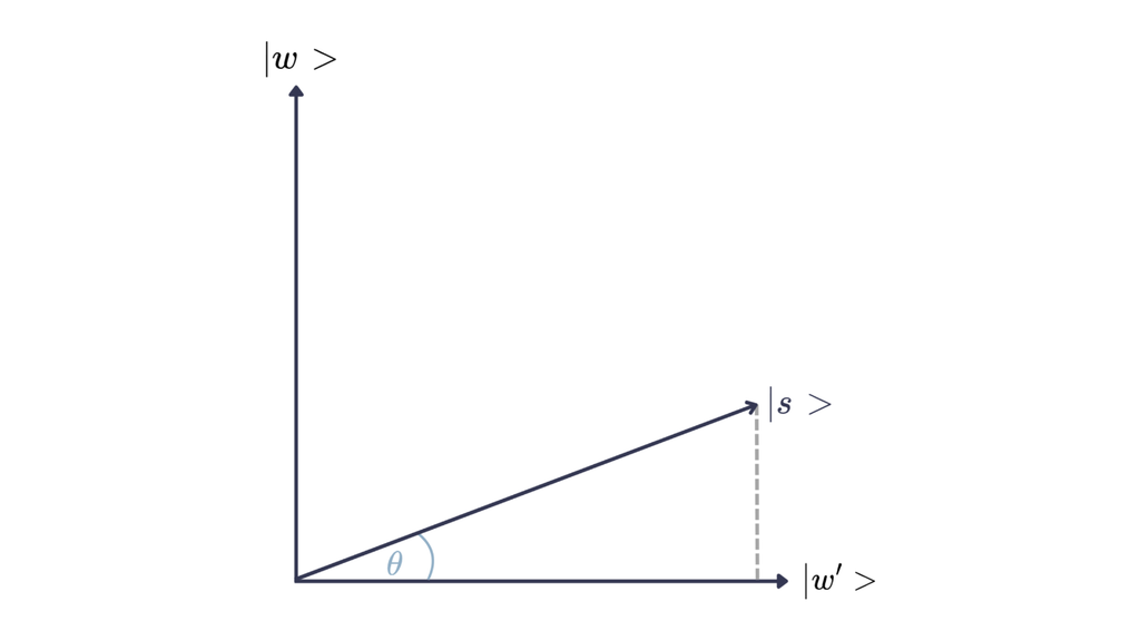
Figure 2 shows the state \(|s>\) together with an angle \(\theta\) that describes the angle between \(|s>\) and the \(|w’>\)-axis.
If we incorporate the dotted line, then the result is a right-angled triangle where the hypotenuse has a length of \(1\), the height corresponds to the share of \(|w>\) in \(|s>\) and the width of the triangle equals the share of \(|w’>\) in \(|s>\).
We can therefore write that \(sin(\theta) = \frac{height}{1} = \frac{\sqrt{M}}{\sqrt{N}}\) and \(cos(\theta) = \frac{width}{1} = \frac{\sqrt{N – M}}{\sqrt{N}}\).
The state as a whole can be stated in dependence of \(\theta\) as \(|s> = \frac{\sqrt{M}}{\sqrt{N}} |w> + \frac{\sqrt{N – M}}{\sqrt{N}} |w’>\) \(= sin(\theta) |w> + cos(\theta) |w’>\).
This representation is, again, a valid quantum state since \(sin^2(x) + cos^2(x) = 1\).
Oracle + Diffusion = Rotation
The oracle in Grover’s algorithm marks all those states with a phase of \(-1\), that satisfy the condition of the search problem. Geometrically, this corresponds to a reflection of the vector of \(|s>\) across the \(|w’>\)-axis: \(O|s> = O(a |w> + b |w’>) = -a |w> + b |w’>\)
The diffusion operator reflects any state it is applied to against the equal superposition state \(\frac{1}{\sqrt{N}} \sum_{i=0}^{N-1}|i>\). Geometrically, this amounts to a reflection across the initial state \(|s>\).
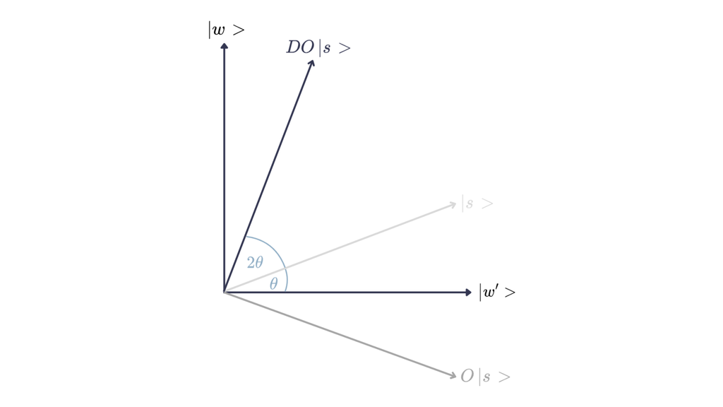
With every iteration of oracle + diffusion, the current state is reflected first on the \(|w’>\)-axis and then across the initial state \(|s>\).
Geometrically, this sequence increases the angle between the current
state and the \(|w’>\)-axis by \(2 \theta\) with every iteration.
The state of the system is moving counter-clockwise, starting near \(|w’>\) and moving towards \(|w>\) in early iterations.
After \(k\) iterations, our system is in a state of \(|s> = sin((2k + 1)\theta) |w> + cos((2k + 1)\theta) |w’>\).
Note, that if the iteration count is chosen too high, we might overshoot our goal and decrease the probability amplitude of the target state \(|w>\) as we rotate further.
So, why the \(\sqrt{N}\)?
Ideally, we would like to stop updating our vector as soon as we reach the \(|w>\)-axis (or at least are very close).
Therefore, we are looking for a \(k\) so that \((2k + 1)\theta \approx \frac{\pi}{2}\).
Using the equivalence that \(sin(\theta) = \frac{\sqrt{M}}{\sqrt{N}}\) we can rewrite \(\theta\) as \(\theta = sin^-1(\frac{\sqrt{M}}{\sqrt{N}})\).
Remembering that \(sin(x) = x\) for small values of \(x\), we can usually assume that \(N >> M\) and therefore rewrite \(sin^{-1}(\frac{\sqrt{M}}{\sqrt{N}}) \approx \frac{\sqrt{M}}{\sqrt{N}}\). This leaves us with \(\theta = \frac{\sqrt{M}}{\sqrt{N}}\).
To maximize the probability amplitude of the correct states, we need to find a \(k\) so that \((2k + 1)\theta \approx \frac{\pi}{2}\). Replacing \(\theta\) with \(\frac{\sqrt{M}}{\sqrt{N}}\), this leaves us with \((2k + 1)\frac{\sqrt{M}}{\sqrt{N}} = \frac{\pi}{2}\).
After rewriting for \(k\), we are left with \(k = (\frac{\pi}{2} * \frac{\sqrt{N}}{\sqrt{M}} – 1) / 2 = \frac{\pi}{4} * \frac{\sqrt{N}}{\sqrt{M}} – \frac{1}{2})\).
The optimal number of iterations in Grover’s algorithm is the whole number that comes closest to \(\frac{\pi}{4} * \frac{\sqrt{N}}{\sqrt{M}} – \frac{1}{2}\).
This number scales with \(O(\frac{\sqrt{N}}{\sqrt{M}})\) and therefore offers a quadratic speedup in \(N\).