The Quantum Fourier Transform (QFT) is one of the most popular and widely used quantum algorithms today. It is part of many other quantum algorithms, including Quantum Phase Estimation and Shor’s Algorithm, and can be seen as a quantum version of the Discrete Fourier Transform (DFT).
While it is easy to show that the Quantum and the Discrete Fourier Transform perform the same operation, why this is the case is a lot less obvious.
In this article, we will derive the circuit of the Quantum Fourier Transform based on the definition of the Discrete Fourier Transform. Afterward, I will highlight some lessons we can take from the QFT regarding quantum algorithms and quantum algorithm development in general.
Let’s dig in!
Note: This article assumes that you have a basic understanding of what a Fourier Transform is and what it does. If you are new to the topic, this video by the Youtube Channel Up and Atom contains a nice introduction.
A prove that QFT and DFT do the same
Mathematically speaking, the DFT is defined as
\( f_k = \sum_{j=0}^{N-1} s_ j \times e^{\frac{2 \pi i \times j k}{N}} \)
The weight of a frequency \( f_k \) in the frequency decomposition of a signal (sequence of all \( s_j \)) is computed as the sum of each sample in the signal (\( s_j \)) times a wave term (\(e^{\frac{2 \pi i \times j k}{N}} \)) dependent on the frequency k and the index of the sample j.
If we represent all samples in the signal as a vector, where the position in the vector equals the index of the sample, the full decomposition of the signal into frequencies can be written as a matrix where each cell contains a power of the wave term \(w = e^{\frac{2 \pi i}{N}} \).
\( DFT = \begin{pmatrix} w^{0 \times 0} & w^{0 \times 0} & … & w^{0 \times (N – 1)} \\ w^{1 \times 0} & w^{1 \times 0} & … & w^{1 \times (N – 1)} \\ … & … & … & … \\ w^{(N – 1) \times 0} & w^{(N – 1) \times 0} & … & w^{(N – 1) \times (N – 1)} \end{pmatrix} \)
In this matrix, the column indices correspond to the position of each sample in the signal, while each row corresponds to a frequency term.
Does that remind you of something?
If we normalize this matrix, it becomes a unitary operation. Each column describes how an input state from the signal domain is mapped to a superposition of all possible output states from the frequency domain.
This normalized matrix, the matrix representation of the Discrete Fourier Transform, is exactly equal to the unitary matrix corresponding to the quantum circuit of the Quantum Fourier Transform:

with \( R_k = \begin{pmatrix} 1 & 0 \\ 0 & e^{\frac{2 \pi i}{2^k}} \end{pmatrix}\).
So, where does the circuit come from?
If an operation is applied to a superposition state, it gets distributed to each of its component states. A single operation can thereby affect multiple states at once, a phenomenon referred to as Quantum Parallelism. (See Is Quantum Computing parallel? for more details.)
In our case, if we encoded the signal we wish to decompose as the coefficients of the individual states of a superposition, we can write the whole operation as
\( |frequencies> = QFT |signal> \)
\( = QFT (c_0 |s_0> + c_1 |s_1> + … + c_{N-1} |s_{N-1}>) \)
\( = c_0 QFT |s_0> + c_1 QFT |s_1> + … + c_{N-1} QFT |s_{N-1}> \)
where \( |s_j> \) is the j-th sample in the signal.
If we pass a superposition state through a quantum circuit, we can think of it as the circuit manipulating each of the individual states in parallel and interferring the results at the end. The circuit of the QFT can be seen as an operation that maps each input state from the signal domain to a superposition of states representing the frequency domain.
Within the corresponding unitary matrix, the value of each cell is computed as \(e^{\frac{2 \pi i \times j k}{N}}\).
If we represent the indices of f and s in binary, we can rewrite the value of each cell \(c_{j,k}\) in the matrix as
\(c_{j,k} = e^{\frac{2 \pi i \times j k}{N}} = e^{\frac{2 \pi i}{N} (\sum_{p=0}^{n-1} s_{j, p} 2^p)(\sum_{q=0}^{n-1} f_{k, q} 2^q) } \),
where \(s_{j,p}\) is the value of the p-th bit of \(s_j\), \(f_{k, q}\) is the value of the q-th bit of \(f_k\), and \(n = log_2(N)\).
This can be rewritten as
\(c_{j,k} = \prod_{p = 0}^{n – 1} 1 \prod_{q = 0}^{n – 1} (e^{\frac{2 \pi i}{N} \times 2^{p+q}})^ {s_{j, p} \times f_{k, q}} \)
In other words: For every bit \(s_{j,p}\) in \(s_{j}\) and every bit \(f_{k, q}\) in \(f_k\), we add a factor of \(e^{\frac{2 \pi i}{N} \times 2^{p+q}}\) if \(s_{j,p}\) and \(f_{k, q}\) are 1.
If either \(s_{j,p}\) or \(f_{k, q}\) equal 0, we add a factor of \((e^{\frac{2 \pi}{N} \times 2^{p+q}})^0 = 1\), which can therefore safely ignore.
Next, we swap the order of the bits in \(f_{k}\). \(f_{k, 0}\) shall correspond to \(2^{n-1}\), \(f_{k, 1}\) to \(2^{n-2}\), and so forth. In general, the q-th bit of \(f_{k}\) now corresponds to \(2^{n-1-q}\) instead of the original \(2^{q}\)*.
* I know, this step may seem arbitrary at first, but bear with me. The beauty of this mathematical trickery will become clear in a second.
After this transformation has been applied, the value of each cell can be expressed as
\(c_{j,k} = \prod_{p = 0}^{n – 1} 1 \prod_{q = 0}^{n – 1} (e^{\frac{2 \pi i}{N} \times 2^{p+ n – 1 – q}})^ {s_{j, p} \times f_{k, q}} \)
\( = \prod_{p = 0}^{n – 1} 1 \prod_{q = 0}^{n – 1} (e^{\frac{2 \pi i}{2^n} \times 2^{p+ n – 1 – q}})^ {s_{j, p} \times f_{k, q}} \)
\( = \prod_{p = 0}^{n – 1} 1 \prod_{q = 0}^{n – 1} (e^{2 \pi i \times 2^{p+ n – 1 – q – n}})^ {s_{j, p} \times f_{k, q}} \)
\( = \prod_{p = 0}^{n – 1} 1 \prod_{q = 0}^{n – 1} (e^{2 \pi i \times 2^{p – q – 1}})^ {s_{j, p} \times f_{k, q}} \)
If \( p > q \), \( 2^{p-q-1} \) turns out to be an integer multiple of 2, resulting in \(e^{2 \pi i \times 2^{p – q – 1}} = 1\).
Therefore, we only have to consider the cases where \( p \leq q \), as all other cases amount in an additional factor of 1. This allows us to rewrite our formula as
\( c_{j,k} = \prod_{p = 0}^{n – 1} 1 \prod_{q = p}^{n – 1} (e^{2 \pi i \times 2^{p – q – 1}})^ {s_{j, p} \times f_{k, q}} \)
Starting to look familiar?
If we define k as \(k = – (p – q – 1) = q – p + 1\), we get
\( c_{j,k} = \prod_{p = 0}^{n – 1} 1 \prod_{q = p}^{n – 1} (e^{2 \pi i \times 2^{-k }})^ {s_{j, p} \times f_{k, q}} \)
\( = \prod_{p = 0}^{n – 1} 1 \prod_{q = p}^{n – 1} (e^{\frac{2 \pi i}{2^k}})^ {s_{j, p} \times f_{k, q}} \)
For every bit p in \( s_{j} \) that is in a state of 1, we add a factor of \( e^{\frac{2 \pi i}{2^k}}\) for every bit q in \( f_{k} \) that is also in a state of 1, where \( p \leq q \) and k is the distance between p and q + 1.
Let’s translate this into the language of quantum circuits:
- “For every bit p in \( s_{j} \) that is in a state of 1, do something” -> Apply a controlled gate where the control qubit is \( s_{j,p} \).
- “Apply a factor if qubit q is is a state of 1” -> Apply a gate that only acts on the |1> state of a qubit. Examples include the Z-Gate, the S-Gate, or in our case, the more generic Phase gate.
In summary: For every qubit of index p, add a controlled phase gate to all qubits with index q > p with a phase factor of \(e^{\frac{2 \pi i}{2^k}}\), where k is the distance between p and q + 1. Lastly, we need to add a swap layer to counteract the redefinition we decided to do earlier.
The resulting circuit is, as promised:
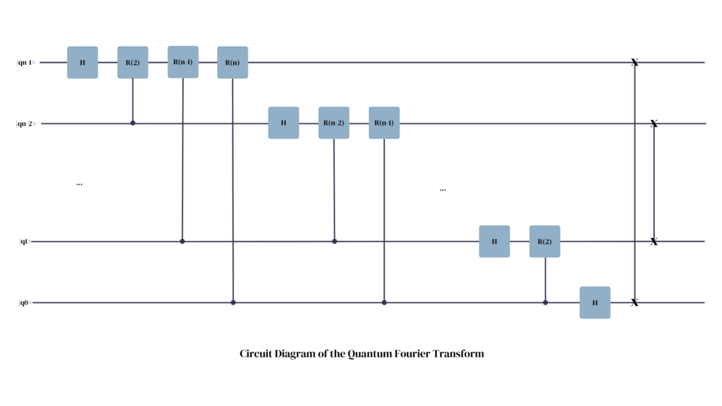
The special case of p = q is covered by the Hadamard gate, since it by default adds a phase factor of -1 (= R(1) ) to the corresponding output qubit if the source qubit was in a state of 1.
General Take Aways
After having done all of the heavy lifting, let’s take a step back and consider what we might learn from this endeavour for quantum algorithm development in general.
Any summation of coefficients can be interpreted as quantum interference of the corresponding states. Representing a summation as matrix, makes it easier to discern how much each input state should contribute to the coefficient of each output state.
A quantum circuit can be seen as a gradual transition from an input state to a superposition of output states. As long as a qubit has not been modified through a gate, it is still in its input state and can therefor be used to control the manipulation of other gates. In the QFT, this is seen in the fact that each qubit acts as a control qubit before being manipulated through Hadamard and phase gates.
Sometimes, redefining what the qubits mean can drastically simplify a calculation. Detecting the situations where that is possible, however, requires a lot of intuition about both math and quantum computing.
At its core, the DFT uses wave functions in the form \( e^{2 \pi i x} \) with \( x \epsilon \mathbb{N}\). Since the absolute value of \(|e^{2 \pi i x}| = 1\), regardless of the value of x, the calculation as a whole has a determinant of 1. While this fact alone does not ensure unitarity, it is an important condition for quantum computerification.
If we manage to detect “traces of unitarity” in other classical algorithms or find ways to map these algorithms to a unitary representation, we could find other quantum algorithms like the QFT in the near future. Who knows…
Summary
In this article, we derived the circuit of the QFT from the mathematical definition of the DFT through a series of mathematical tricks and transformations. The resulting quantum circuit provides a method to speed up the computation of a DFT through the use of quantum superposition and interference.
While there are still comparatively few quantum algorithms out there, the steps we took to get from the DFT to the QFT can serve as a blueprint for detecting and transforming other (non-quantum) algorithms in the future.